



Introduction
Every year, trillions of dollars flow into large-scale industrial infrastructure projects — power grids, pipelines, offshore platforms, highways, and desalination plants. Yet, despite rigorous feasibility studies, a striking number of these projects arrive over budget, behind schedule, or financially impaired. The root cause is almost never negligence. Instead, it is a systematic failure to model uncertainty with the mathematical precision that modern operations research demands.
Traditionally, investment appraisal relies on deterministic tools: a fixed discount rate, a single revenue forecast, a point-estimate for construction costs. While these tools are useful as a starting point, they are fundamentally incomplete. They describe only one possible future — the most likely one. However, in practice, infrastructure investments unfold across one, two, or three decades of volatile commodity prices, shifting regulatory landscapes, and unpredictable demand patterns. A single forecast is not a strategy; it is an illusion of certainty.
This is precisely where Monte Carlo simulations for infrastructure investment risk enter the equation. Originally developed during the Manhattan Project by mathematicians Stanislaw Ulam and John von Neumann in the 1940s, the Monte Carlo method uses random sampling to model the behavior of complex systems across thousands — or even millions — of simulated outcomes. When applied to capital budgeting and project risk analysis, it transforms a static Net Present Value (NPV) figure into a rich probability distribution, empowering decision-makers with statistically grounded confidence intervals rather than false certainties.
This article explores the full application of Monte Carlo simulation in large-scale industrial infrastructure investment decisions. We will examine the mathematical foundations, the process of building a credible simulation model, and the methods for interpreting and acting on the results. Furthermore, we will consider the critical integration of this technique with complementary tools from operations research, such as sensitivity analysis and real options theory, to present a genuinely robust quantitative risk framework.
Can Monte Carlo Simulation Really Predict Whether a $2 Billion Infrastructure Project Will Fail?
1. The Mathematical Foundation: From Deterministic NPV to Probabilistic Distributions
To understand the power of Monte Carlo simulation, one must first appreciate the limitations of the models it replaces. The conventional Net Present Value approach discounts all expected future cash flows back to the present using a fixed weighted average cost of capital (WACC). The resulting single number — the NPV — is then used to approve or reject an investment. A positive NPV signals value creation; a negative NPV signals destruction.
The problem, as the renowned economist Frank Knight observed, lies in the fundamental difference between “risk” and “uncertainty.” Risk is quantifiable through historical probabilities. Uncertainty, on the other hand, describes situations where the distribution of outcomes is itself unknown — a condition that perfectly characterizes long-horizon infrastructure investments 1 . The classic deterministic NPV model handles risk poorly and handles uncertainty not at all.
“Whereas engineers calculate with numbers, the real uncertainty is that the model itself may be wrong. The map is not the territory.”— Nassim Nicholas Taleb, The Black Swan (2007)
Monte Carlo simulation directly addresses this limitation. Instead of assigning a single value to each variable (e.g., a fixed oil price of $85/barrel), the analyst assigns a probability distribution to each uncertain input. For instance, oil prices might follow a log-normal distribution with a mean of $85 and a standard deviation of $15. Construction costs might follow a triangular distribution with a minimum of $1.8 billion, a most likely value of $2.1 billion, and a maximum of $2.7 billion.
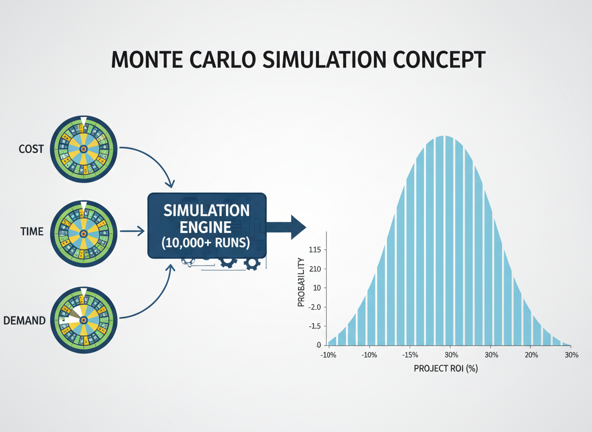
The simulation engine then executes tens of thousands of iterations. In each iteration, it randomly samples a value from every input distribution, computes the resulting NPV (or Internal Rate of Return, or any target metric), and records the output. After completing all iterations, the recorded outputs form a probability distribution of outcomes — a histogram that answers not just “what is the expected NPV?” but “what is the probability that this project destroys value?” or “what NPV can we achieve with 90% confidence?” 2 .
The mathematics underpinning this approach are grounded in the Law of Large Numbers and the Central Limit Theorem. As the number of simulations increases, the distribution of the mean output converges toward the true expected value of the system. For complex systems with non-linear interactions between variables — exactly the type of systems found in large industrial projects — the Monte Carlo method provides results that are analytically intractable through closed-form mathematical solutions. It is, in essence, a computational substitute for an equation that cannot be solved algebraically.
“All models are wrong, but some are useful.”— George E.P. Box, statistician
In my professional view, the single most valuable output of a Monte Carlo simulation is not the mean expected NPV — it is the shape of the full distribution. A distribution that is wide and spread out tells the decision-maker that this project carries enormous outcome variance; the upside may be extraordinary, but so is the risk of catastrophic loss. A narrow distribution clustered around positive values communicates a resilient project. This shape, this “fingerprint” of a project’s risk profile, is invisible to deterministic models and is precisely the information that boards of directors, infrastructure lenders, and public regulators most urgently need.
2. Building a Credible Simulation Model for Industrial Projects
The quality of a Monte Carlo simulation model is entirely dependent on the quality of its inputs. This principle — “garbage in, garbage out” — is especially consequential in high-stakes infrastructure contexts, where the outputs of the model directly influence billion-dollar capital allocation decisions. Therefore, building a credible model is a disciplined, multi-step process that combines financial modeling, domain expertise, statistical reasoning, and a healthy respect for the limits of quantification.
The first step is variable identification. The analyst must identify every material uncertain input that affects the project’s financial outcomes. For a large-scale liquefied natural gas (LNG) terminal, for example, relevant uncertain variables typically include: initial capital expenditure (CAPEX), annual operational expenditure (OPEX), LNG spot price and forward curve, throughput volume and offtake contract execution rate, construction timeline and associated delay penalties, financing interest rates, and the probability and magnitude of regulatory or environmental compliance costs 3 .

The second step is distribution fitting. Once variables are identified, the analyst must assign appropriate probability distributions to each. This process should be grounded in empirical data wherever possible — historical commodity price series, engineering cost databases, project delivery benchmarks, and actuarial risk registers. When historical data is scarce (as is common for novel technologies or unprecedented regulatory environments), expert elicitation methods, such as the Delphi technique, are used to extract structured probabilistic judgments from domain experts 4 .
Common distribution types used in infrastructure models include: triangular distributions (defined by minimum, most likely, and maximum values — useful for cost estimates where engineering judgment is primary); log-normal distributions (suitable for strictly positive variables like commodity prices that exhibit right-skewed behavior); normal distributions (appropriate for aggregated variables governed by the Central Limit Theorem, such as portfolio revenues); and discrete distributions or Bernoulli trials (for binary risk events like permit approval or force majeure). The practitioner must choose distributions thoughtfully, as the shape assumption meaningfully affects the tail risk of the output distribution.
“Give me six hours to chop down a tree and I will spend the first four sharpening the axe.”— Abraham Lincoln
The third and often most technically demanding step is correlation modeling. In reality, many risk variables do not move independently. Commodity prices, inflation rates, and OPEX costs may be positively correlated. Macroeconomic downturns may simultaneously depress throughput demand and tighten financing conditions. A simulation model that treats all variables as independent will dramatically underestimate tail risk — the very scenarios that threaten project viability. Correlation is typically modeled using a Cholesky decomposition of the correlation matrix or through copula functions for more complex dependency structures. From an operations research standpoint, this step is non-negotiable for any model that aspires to professional credibility.
The fourth step is model validation. Before the simulation is run for decision purposes, the model should be validated through back-testing (comparing outputs to historical project outcomes), stress testing (examining behavior under extreme but plausible scenarios), and peer review by independent quantitative analysts. This validation discipline mirrors the rigor applied to models in regulated financial institutions — and it is equally necessary in industrial infrastructure contexts, where governance standards are increasingly demanding that quantitative risk models be documented, audited, and traceable to their underlying assumptions.
3. Interpreting Results and Integrating with Real Options Analysis
Once a Monte Carlo simulation has been executed — typically using specialized software such as Oracle Crystal Ball, @RISK (Palisade), MATLAB, or custom Python environments using libraries like NumPy and SciPy — the analyst is confronted with a wealth of statistical output. Transforming this output into actionable strategic intelligence requires a clear interpretive framework.
The primary output metric is the probability distribution of the project NPV. From this distribution, the analyst extracts several critical statistics: the expected (mean) NPV, the median NPV, the standard deviation, the probability that NPV is negative (i.e., P(NPV < 0)), and the 10th and 90th percentile values (the P10 and P90 bounds). Together, these statistics define the “risk corridor” of the investment. A project with an expected NPV of +$350 million but a P(NPV < 0) of 38% is a fundamentally different proposition from a project with the same expected NPV but a P(NPV < 0) of only 7%.

A particularly powerful interpretive tool is the tornado chart, produced by sensitivity analysis. This chart ranks each input variable by its contribution to the variance of the output. In essence, it answers the question: “Which uncertain variables drive most of the risk in this project?” For a pipeline project, the tornado chart might reveal that LNG spot price accounts for 52% of NPV variance, CAPEX overrun accounts for 31%, and all other variables are collectively responsible for the remaining 17%. This insight is operationally vital: it tells management precisely where risk mitigation efforts and contractual protections should be concentrated.
“The risk of a wrong decision is preferable to the terror of indecision.”— Maimonides, 12th-century philosopher and scholar
The full power of the Monte Carlo framework becomes apparent when it is integrated with Real Options Analysis (ROA). Real options theory, pioneered by Stewart Myers at MIT in 1977, recognizes that capital investments embed managerial flexibilities that have quantifiable value. The option to abandon a project if early-phase performance is below threshold, the option to expand capacity if demand exceeds projections, and the option to delay a construction commitment until regulatory clarity is achieved — all of these are financial options that a deterministic NPV model assigns a value of zero.
When a Monte Carlo simulation generates a full probability distribution of future project states, it provides precisely the volatility parameters that real options pricing models require. The Black-Scholes framework or binomial lattice models can then be applied to price these embedded flexibilities, revealing that the total project value equals the static NPV plus the value of real options. For large-scale infrastructure projects with multi-decade horizons, the value of embedded managerial options can materially exceed the static NPV — and in borderline cases, may be the deciding factor in whether a project should proceed, be restructured, or be staged with contingent milestones.
From a strategic operations research perspective, this integrated quantitative framework — Monte Carlo simulation for infrastructure investment risk, tornado sensitivity analysis, and real options valuation — represents the current frontier of rigorous industrial investment appraisal. It is no longer the domain of academia alone. Leading infrastructure developers, sovereign wealth funds, and multilateral development banks have progressively embedded these methods into their formal investment governance processes. The question today is not whether to use them, but how to use them with sufficient discipline and transparency to satisfy the scrutiny of boards, regulators, and lenders.
Conclusion
“It is not the strongest of the species that survives, nor the most intelligent, but the one most responsive to change.”— Charles Darwin (attributed)
Large-scale industrial infrastructure investment is, by its very nature, an exercise in making consequential commitments under profound uncertainty. The deterministic tools that dominated capital budgeting for decades — static NPV, break-even analysis, scenario tables — are not wrong, but they are insufficient. They present decision-makers with a mirage of precision that masks the true probabilistic nature of long-horizon projects.
Monte Carlo simulations for infrastructure investment risk offer a mathematically honest and operationally powerful alternative. By replacing point estimates with probability distributions, executing thousands of independent simulations, and presenting the results as a full distribution of possible outcomes, the Monte Carlo method gives engineers, executives, lenders, and regulators a genuinely informative view of what they are committing to. It does not eliminate uncertainty — nothing can — but it makes uncertainty visible, measurable, and manageable.
When this method is combined with rigorous correlation modeling, sensitivity-based tornado analysis, and the real options framework, the result is a quantitative investment governance architecture that meets the highest standards of modern operations research. Moreover, it aligns with the emerging expectations of regulatory frameworks and international accounting standards that increasingly require probabilistic disclosures in major capital project assessments.
The world urgently needs high-quality infrastructure. The energy transition, the digital economy, the demands of a growing global population — all of these forces are converging to require trillions in new capital investment. In this context, better risk quantification is not a merely academic exercise. It is a strategic imperative. Projects that are well-modeled are better financed, better governed, and more likely to deliver their intended economic and social value. The Monte Carlo method, applied with discipline and intellectual honesty, is one of the most powerful tools engineers and financial professionals possess to rise to that challenge.
“In God we trust. All others must bring data.”— W. Edwards Deming, statistician and quality management pioneer