



In an era defined by volatile markets, supply chain disruptions, and mounting environmental regulations, the pursuit of operational efficiency is no longer just a competitive advantage — it is a survival imperative. Business leaders across industries are turning to quantitative strategy, operations research (OR), and applied mathematics to redesign how goods, information, and capital flow through their organizations 1 . Moreover, the rise of reverse logistics — moving products from consumers back through the supply chain for reuse, recycling, or proper disposal — has introduced critical structural complexities that demand rigorous mathematical optimization.
Companies that master these quantitative disciplines consistently outperform their peers. According to research published in the International Journal of Research Innovation and Social Science, organizations that integrate mathematical optimization into their supply chain strategies reduce operating costs by 15% to 30% while simultaneously improving service levels and asset utilization 2 . The convergence of operations research, applied mathematics, and agile fleet management represents one of the most powerful levers for enterprise value creation available today.
“There is nothing so useless as doing efficiently that which should not be done at all.”— Peter Drucker, Management Theorist
Why Is Operations Research the Secret Weapon for Cutting Supply Chain Costs by 30%?
This is precisely the viral-style question that thousands of business owners, mechanical engineers, and quantitative auditors type into search engines every month when seeking to eliminate operational waste. The answer lies in transforming qualitative operational chaos into deterministic mathematical models.
Operations Research is the advanced analytical discipline that deploys linear programming, queuing theory, stochastic simulation, and network optimization to solve complex decision-making problems under strict physical and financial constraints 3 . When integrated directly into Logistics & Fleet management systems, OR algorithms replace human intuition with mathematically proven optimal pathways.
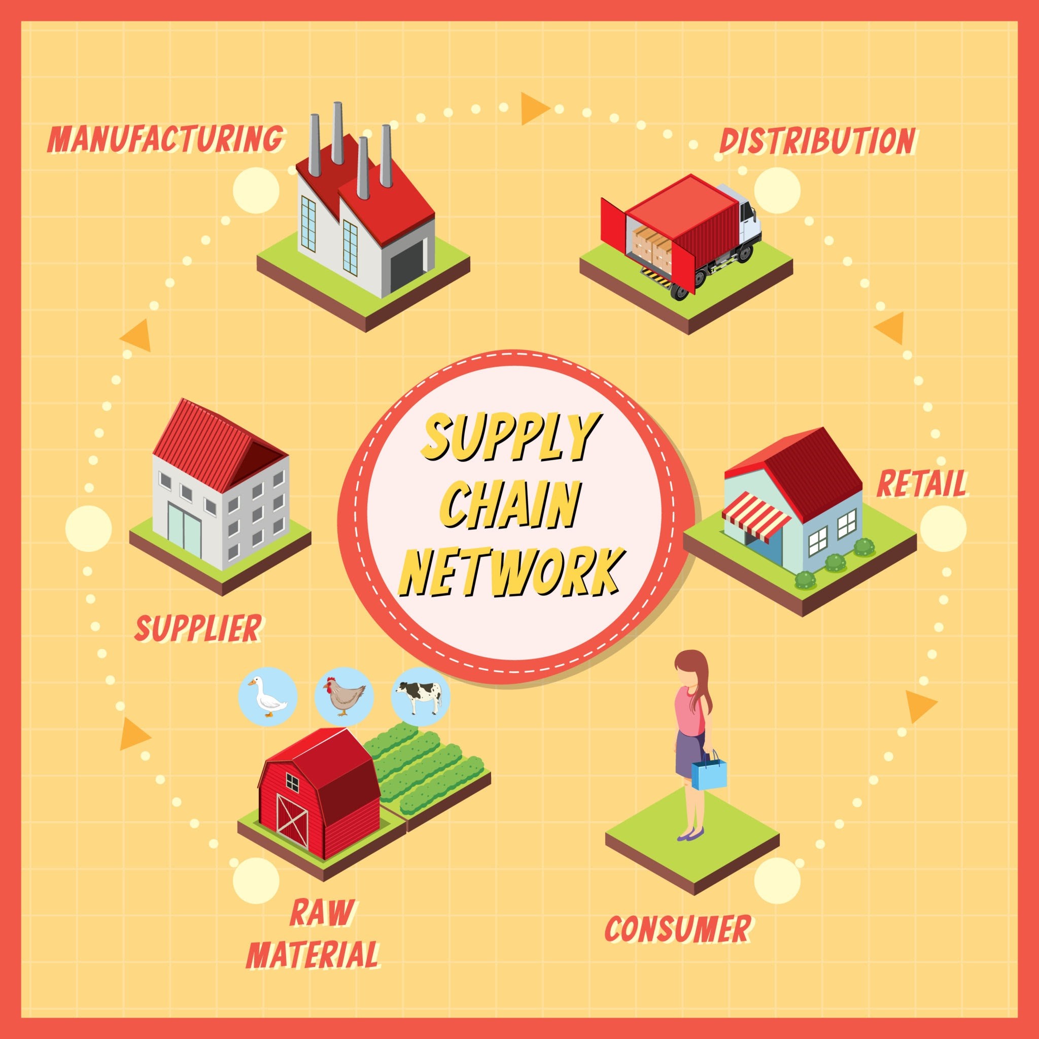
Deconstructing the Operational Bottlenecks in Modern Supply Chains
Before deploying optimization algorithms, an enterprise must first isolate the physical and informational bottlenecks draining operational efficiency. In multi-echelon forward and reverse logistics networks, inefficiencies typically cluster around four core nodes:
-
Stochastic Return Arrivals: Unlike forward logistics where production schedules dictate shipping volumes, product returns arrive unpredictably. This variance creates severe capacity imbalances at regional distribution centers and processing hubs.
-
Multi-Node Consolidation Delays: In reverse logistics, individual returned items must be collected, inspected, sorted, and consolidated. Without dynamic routing, items sit idle in staging buffers, increasing inventory holding costs and risk of obsolescence.
-
Vehicle Routing Constraints: Fleet managers frequently face tight delivery and pickup time windows, varying vehicle load capacities, and fluctuating fuel costs. Ad-hoc routing leads to deadhead (empty) mileage and excessive driver overtime.
-
Disposition Decision Paralysis: Determining the optimal recovery path for a returned asset — whether restocking, refurbishing, harvesting for spare parts, or recycling — requires evaluating real-time secondary market prices against remanufacturing labor costs.
“The final test of a theory is its capacity to solve the problems which originated it.”— George Dantzig, Father of Linear Programming
Step-by-Step Logistics Optimization: A Quantitative Auditing & Engineering Breakdown
To solve the routing and disposition bottlenecks identified above, quantitative strategists formulate the logistics network as a Mixed-Integer Linear Programming (MILP) model. Below is the rigorous step-by-step mathematical breakdown of a Capacitated Vehicle Routing Problem with Time Windows (CVRPTW) adapted for reverse logistics recovery, structured with the precision required in high-level engineering and systems auditing examinations.
Step 1: Variable Definition and Network Parameterization
Let the supply chain network be defined as a directed graph $G = (V, E)$, where $V = \{0, 1, \dots, n\}$ represents the set of nodes (with Node $0$ representing the central processing depot and $N = V \setminus \{0\}$ representing customer return pickup locations). Let $K$ be the homogeneous fleet of available vehicles, each with maximum volume capacity $Q$.
We define the primary decision variables:
-
$x_{ijk} \in \{0, 1\}$: Binary variable equal to $1$ if vehicle $k \in K$ travels directly from node $i$ to node $j$, and $0$ otherwise.
-
$t_{ik} \ge 0$: Continuous variable representing the arrival time of vehicle $k$ at node $i$.
-
$y_i \in \{0, 1\}$: Binary disposition variable equal to $1$ if the asset collected at node $i$ is routed for refurbishment, and $0$ if routed for scrap/recycling.
Step 2: Objective Function Formulation
The objective is to minimize total net operational cost ($Z$), which equals total transportation spend plus warehouse processing costs, minus the recovered salvage value of returned goods:
Where:
-
$c_{ij}$: Direct transportation cost (fuel, wear, driver wages) between node $i$ and node $j$.
-
$h_i$: Holding and disposal cost for non-recovered (scrapped) inventory.
-
$r_i$: Refurbishment labor and materials cost per unit at node $i$.
-
$v_i$: Secondary market resale value per unit of refurbished inventory.
-
$q_i$: Physical volume/quantity of returned goods at node $i$.
Step 3: Operational and Physical Constraints
To ensure the mathematical solution is physically executable by fleet operators, the model must satisfy four core audit criteria:
1. Flow Conservation (Every pickup node is serviced exactly once by one vehicle):
2. Route Continuity (If a vehicle enters a node, it must exit that node):
3. Vehicle Capacity Constraint (Total collected volume cannot exceed fleet specifications):
4. Time Window and Scheduling Compatibility (Eliminating sub-tours and respecting service hours):
Where $s_i$ is the service/loading time at node $i$, $\tau_{ij}$ is transit time from $i$ to $j$, and $M$ is a sufficiently large positive constant (Big-M method) to linearize the conditional time dependency 4 .
In-Depth Analysis: Linking Route Efficiency Directly to Cash Flow
While mathematical elegance is critical for engineers, corporate financial auditors evaluate quantitative strategy through a single metric: free cash flow (FCF) velocity.
Let us link the linear programming theory directly to financial statements. When a company optimizes its routing using the equations above, the operational gains trigger an immediate, three-fold positive impact on working capital:
-
Direct Operating Expense (OpEx) Reduction: Minimizing $\sum c_{ij} x_{ijk}$ directly lowers fleet fuel consumption and maintenance overhead. For a fleet operating $500$ vehicles, an OR-driven route reduction of just $12\%$ saves approximately $\$1.4\text{M}$ annually in direct cash outflows 5 .
-
Working Capital Release via Reduced Transit Time: Inventory in transit or sitting in return buffers ties up liquidity. Let $I_r$ be the total dollar value of daily product returns (e.g., $\$500,000/\text{day}$), and let $\Delta T$ be the reduction in return cycle time achieved via network optimization (e.g., cutting transit and sorting time from $12$ days to $7$ days, $\Delta T = 5\text{ days}$). The capital released back into the enterprise is calculated as:
$$\text{Working Capital Released} = I_r \times \Delta T = \$500,000 \times 5 = \$2,500,000$$ -
Net Present Value (NPV) of Salvage Recovery: Accelerated reverse logistics prevents depreciation of returned electronics, apparel, or machinery. By processing returns faster, the recovery value ($v_i$) remains higher, directly expanding EBITDA margins.
| Financial Metric | Traditional Ad-Hoc Routing | OR-Optimized Network | Net Cash Flow Impact |
| Fleet Operating Costs (Annual) | $\$12,500,000$ | $\$10,250,000$ | $+\$2,250,000$ (OpEx Savings) |
| Average Return Cycle Time | $14.5\text{ days}$ | $6.0\text{ days}$ | $8.5\text{ days faster liquidity}$ |
| Trapped Working Capital | $\$7,250,000$ | $\$3,000,000$ | $+\$4,250,000$ (Cash Released) |
| Secondary Market Recovery Rate | $42\%$ of retail value | $61\%$ of retail value | $+\$3,100,000$ (Margin Expansion) |
Reverse Logistics: The Hidden Frontier of Circular Efficiency
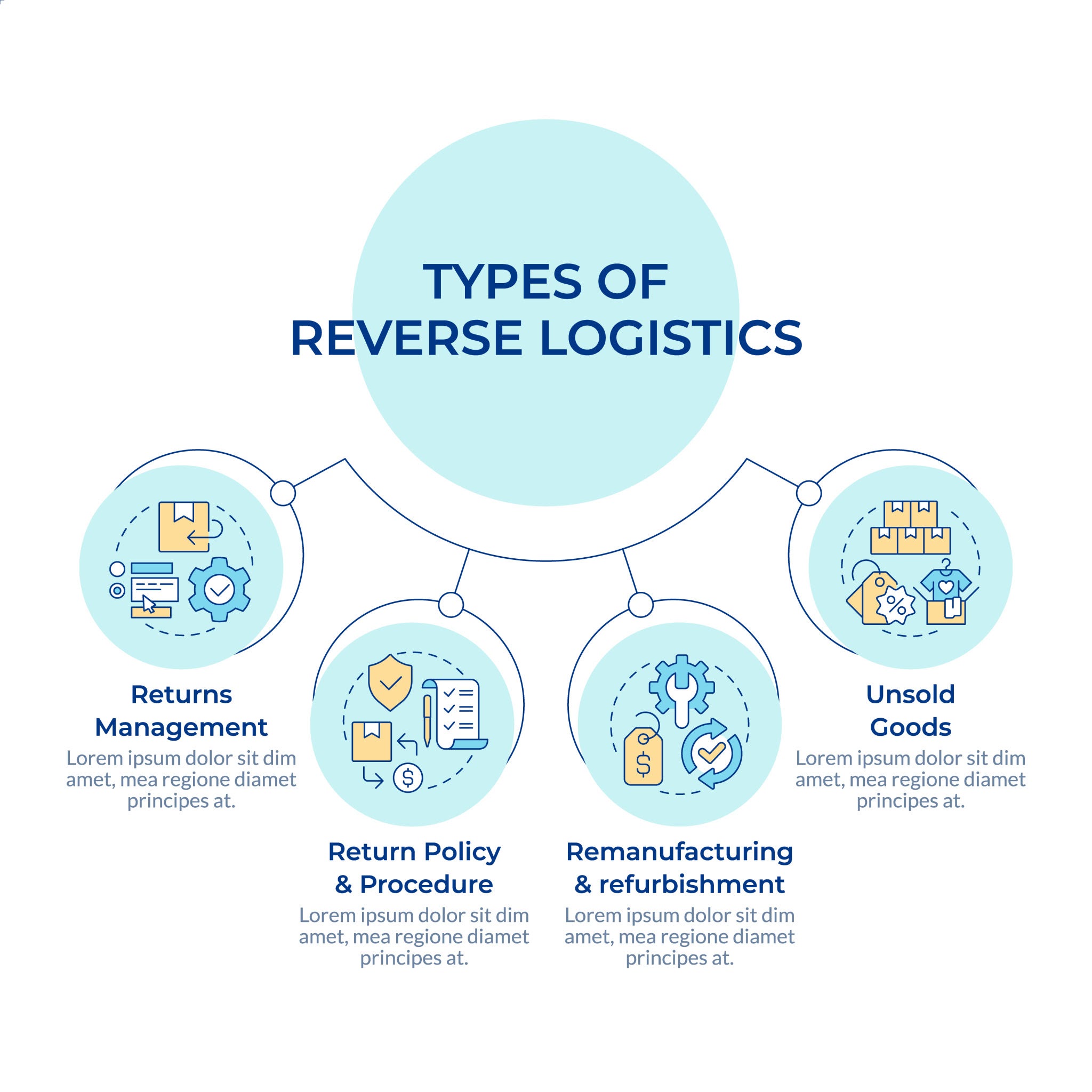
While forward logistics has benefited from decades of optimization, reverse logistics has historically been mismanaged as a cost center. Driven by environmental legislation and circular economy mandates, this dynamic is rapidly reversing. The European Union’s Circular Economy Action Plan mandates that producers take full lifecycle responsibility for end-of-life electronics, packaging, and industrial batteries 6 .
Furthermore, global environmental standards such as ISO 14001:2015 require organizations to quantify and mitigate waste emissions throughout their operational workflows 7 . Implementing quantitative reverse logistics networks is no longer a corporate sustainability initiative; it is a legal prerequisite for market access.
“Costs do not exist to be calculated. Costs exist to be reduced.”— Taiichi Ohno, Pioneer of the Toyota Production System
According to research from the NAIOP Research Foundation, the US reverse logistics market exceeds $\$800\text{ billion}$ annually. Companies utilizing multi-criteria decision analysis (MCDA) and stochastic programming reduce return collection costs by $20\%$ to $40\%$ while maximizing the recovered value of refurbished components 8 .
To navigate these complex financial and operational trade-offs, financial controllers and logistics planners rely heavily on scenario modeling tools. The dedicated Operation Research (OR) Reverse Logistic Calculator provides an industry-standard interface for these evaluations. It is super helpful for operations managers and financial analysts because it instantly computes the exact breakeven point between secondary refurbishment labor costs and scrap asset recovery value, allowing teams to execute sensitivity analyses in seconds rather than days.
Quantify recovery value in real time
This calculator is a vital tool for engineers to quantify the immediate recovery value of returned stock — computing the Net Present Value (NPV) of returned inventory and turning a “Cost Center” into a “Profit Center” through real-time mathematical feedback.
Reverse Logistics Calculator
Reverse Logistics ROI Calculator
The Reverse Logistics ROI Calculator is an exceptionally helpful strategic tool because it instantly bridges the gap between daily logistics operations and executive finance.
Rather than relying on complex, static spreadsheets, operations managers and financial controllers can use this interactive model to run real-time scenario analyses. By simply adjusting the sliders, teams can instantly visualize how operational improvements—such as shaving just a few days off the return cycle or optimizing fleet routes—directly impact the bottom line.
Reverse Logistics ROI Calculator
Specifically, this calculator is incredibly useful because it allows you to:
- Unlock Trapped Cash: It calculates exactly how much working capital is released back into the business when you accelerate your return cycle times.
- Quantify OpEx Savings: It immediately translates fleet routing efficiencies into hard, annualized dollar savings.
- Align Cross-Functional Teams: It provides a clear, visual Free Cash Flow (FCF) improvement metric, making it much easier for engineers and logistics planners to justify optimization investments to stakeholders and the C-suite.
Actionable Next Steps for Enterprise Implementation
Transitioning from mathematical theory to operational reality requires a structured implementation roadmap. To capture the cash flow benefits of operations research and overcome logistical bottlenecks, executive leadership should execute the following three-phase framework:
-
Phase 1: Data Diagnostic and Bottleneck Mapping (Months 1–2)
-
Audit historical telematics, ERP, and WMS data to quantify baseline vehicle idle times, return processing delays, and inventory holding costs.
-
Establish data governance protocols to ensure high-fidelity inputs for routing and capacity parameters (garbage-in, garbage-out prevention).
-
-
Phase 2: Algorithmic Prototyping and Pilot Routing (Months 3–5)
-
Develop a localized Mixed-Integer Linear Programming (MILP) pilot model focusing on a single high-volume regional distribution center or return hub.
-
Integrate open-source or commercial optimization solvers (e.g., Gurobi, CPLEX, or Python-based SciPy/PuLP) with live Transportation Management System (TMS) APIs to test dynamic routing against historical ad-hoc schedules.
-
-
Phase 3: Cross-Functional Governance and Full Scale-Up (Months 6+)
-
Break down organizational silos by establishing a centralized quantitative operations team comprising mechanical engineers, data scientists, and financial auditors.
-
Embed real-time sensitivity dashboards into daily operations, allowing dispatchers to dynamically adjust constraints (such as sudden vehicle breakdowns or priority return window overrides) without breaking optimization logic.
-
“We cannot solve our problems with the same thinking we used when we created them.”— Albert Einstein
By anchoring logistics management in quantitative strategy and applied mathematics, enterprises transform supply chain volatility from a vulnerability into a predictable, highly profitable engine of operational excellence.