


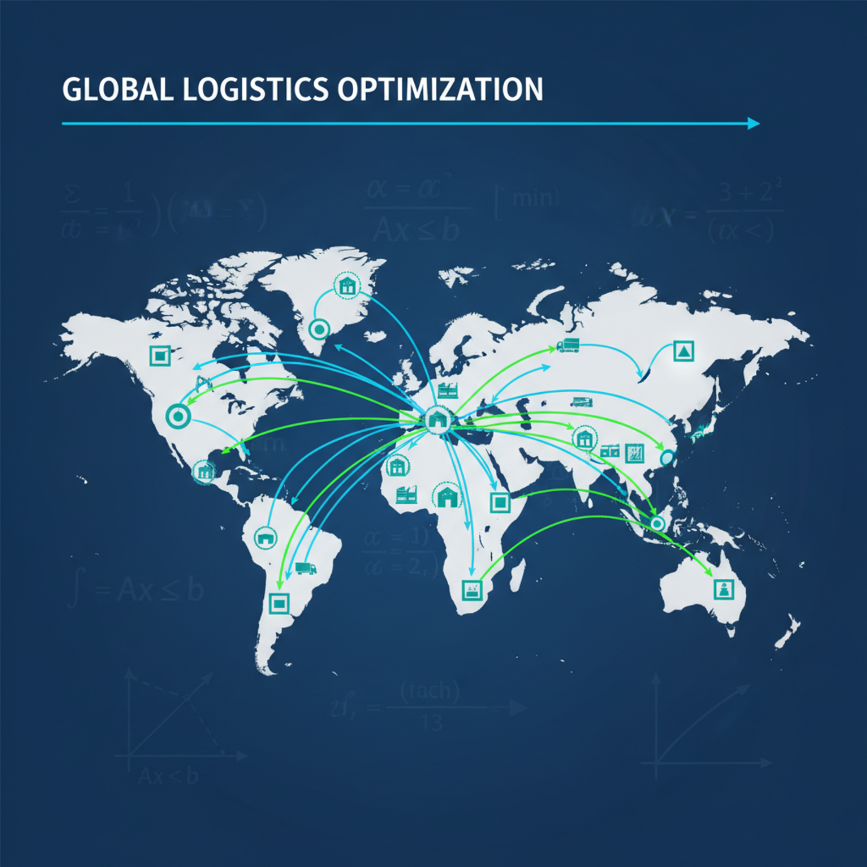
In today’s hyper-competitive global economy, the difference between a market leader and a struggling enterprise lies in the quantitative precision of its supply chain architecture. Operations Research (OR)—the application of advanced mathematical modeling, optimization, and stochastic analysis—has become the primary driver of operational efficiency in high-performance distribution networks.
With U.S. business logistics costs reaching $2.58 trillion, representing approximately 8.8% of national GDP 1 , the financial leverage of logistics optimization is immense. For global operations, exploring specialized analytical methodologies within our Logistics & Fleet subcategory reveals how cutting-edge quantitative models translate directly into balance sheet performance.
“The goal is to turn data into information, and information into insight.”— Carly Fiorina, former CEO of Hewlett-Packard
Operational Bottlenecks in Traditional Supply Chain Architecture
Before deploying mathematical optimization models, quantitative strategists must identify and isolate systemic operational friction points. Unoptimized distribution networks consistently suffer from structural inefficiencies that impair throughput and inflate capital expenditure:
-
Cross-Dock & Facility Bottlenecks: Suboptimal dock door allocation, poor inventory slotting, and uncoordinated staging schedules lead to extended dwell times and labor overhead.
-
Asymmetric Fleet Underutilization: Static routing algorithms produce severe empty-mile ratios, suboptimal vehicle volume fill rates, and inflated fuel consumption.
-
Stochastic Lead-Time Variance: Unhedged variability in multi-modal transit legs forces excess safety stock buffering, locking up millions in non-earning working capital.
-
Combinatorial Last-Mile Complexity: Exponential expansion of delivery nodes creates severe routing inefficiencies when managed via human intuition or simple heuristic methods.
-
Reverse Logistics Network Inefficiencies: Unstructured return pipelines create backlogs in value recovery, re-manufacturing, and compliant disposal.
1. Mathematical Foundations of Logistics Optimization
At the core of modern quant logistics is the transition from static heuristics to dynamic, exact mathematical programming.
“In God we trust. All others must bring data.”— W. Edwards Deming, statistician and quality management pioneer
Formal Optimization Breakdown: Multi-Echelon Facility & Flow Allocation
To evaluate a supply chain network deterministically, consider a Mixed-Integer Linear Programming (MILP) formulation for a multi-echelon network consisting of candidate Distribution Centers (DCs) $I$ serving regional demand zones $J$.
Step 1: Decision Variable & Parameter Definitions
-
$y_i \in \{0, 1\}$: Binary variable indicating if candidate DC $i \in I$ is operational.
-
$x_{ij} \ge 0$: Continuous variable representing shipment volume from DC $i \in I$ to customer zone $j \in J$.
-
$f_i$: Annual fixed operational expenditure (OpEx) for opening DC $i$ ($\$$).
-
$c_{ij}$: Unit transportation cost from DC $i$ to customer zone $j$ ($\$/\text{unit}$).
-
$h_j$: Unit inventory holding cost rate at zone $j$ ($\$/\text{unit}$).
-
$d_j$: Deterministic demand at customer zone $j$ ($\text{units}$).
-
$K_i$: Throughput capacity limit of candidate DC $i$ ($\text{units}$).
Step 2: Objective Function Construction
The primary objective is to minimize total operational cost ($Z$), encompassing fixed facility costs and variable transportation/holding expenses:
Step 3: Operational Constraints
-
Demand Satisfaction Constraint: Ensures every demand zone receives its required throughput:
$$\sum_{i \in I} x_{ij} \ge d_j \quad \forall j \in J$$ -
Capacity Constraint: Restricts flow through DC $i$ to zero if closed, and to $K_i$ if open:
$$\sum_{j \in J} x_{ij} \le K_i y_i \quad \forall i \in I$$ -
Integrality & Non-Negativity Constraints:
$$y_i \in \{0, 1\} \quad \forall i \in I, \quad x_{ij} \ge 0 \quad \forall i \in I, j \in J$$
In complex environments, such as McDonald’s China deployment across 6,000+ restaurants 2 , these exact formulations reduce network cost structures dramatically while increasing Service Level Agreement (SLA) reliability. Furthermore, deploying advanced Vehicle Routing Problem (VRP) algorithms yields route efficiency gains that systematically reduce operational fleet costs by 15% to 30% 3 .
Financial Impact Analysis: Linking Route Optimization to Cash Flow
Theoretical route optimization directly alters financial metrics. By minimizing total ton-mileage and network transit time, an organization achieves significant cash flow acceleration across key metrics:
| QUANTITATIVE CASH FLOW IMPACT | |
| Operational Efficiency Metric | Direct Financial / Balance Sheet Impact |
| Ton-Mile Reduction (15% – 25%) | Decreases COGS; immediate boost to EBITDA |
| Safety Stock Minimization | Reduces tied-up Working Capital in $SS$. |
| Days Inventory Outstanding (DIO) | Shortens Cash Conversion Cycle (CCC). |
| Dynamic Fleet Routing Optimization | Lowers CapEx (fleet expansion deferred). |
Mathematically, safety stock ($SS$) reduction under variable demand ($\sigma_D$) and lead time variability ($\sigma_L$) directly releases working capital:
Reducing lead time variance ($\sigma_L$) through OR-driven multi-modal route stabilization lowers $SS$ requirements exponentially, directly increasing Free Cash Flow (FCF).
2. Global Distribution Networks: Design, Simulation, and Real-Time Control
“The essence of mathematics is not to make simple things complicated, but to make complicated things simple.”— Stan Gudder, mathematician
Modern supply chain network design (SCND) integrates static MILP solutions with real-time discrete-event simulation. By linking operational telemetry from fleet assets—detailed across our Logistics & Fleet intelligence hub—with IoT tracking architectures, companies transform static planning models into adaptive digital twin ecosystems 4 .
| Real-Time IoT Sensors (GPS, Telematics) | ➜ | MILP / Heuristic (Optimization Model) | ➜ | Real-Time Dynamic Flow (Rerouting & Balancing) |
This dynamic re-balancing is further driven by international trade regulatory realities. For example, compliance under the World Trade Organization’s (WTO) Trade Facilitation Agreement (TFA) demands streamlined customs data interchange 6 . Optimizing cross-border logistics requires including tariff structures, customs delays, and trade barriers as stochastic variables within the primary objective function 5 .
3. Reverse Logistics and the Circular Economy: Optimization Beyond the Last Mile
“There is no such thing as ‘away.’ When we throw anything away, it must go somewhere.”— Annie Leonard, sustainability advocate and author
With regulatory mandates tightening globally—such as the European Union’s Ecodesign for Sustainable Products Regulation (ESPR) 7 and the U.S. Resource Conservation and Recovery Act (RCRA)—reverse logistics is no longer a cost center; it is a mathematical recovery puzzle. For a deeper dive into how this impacts profitability, explore our Logistics & Fleet insights on reverse logistics and business efficiency.
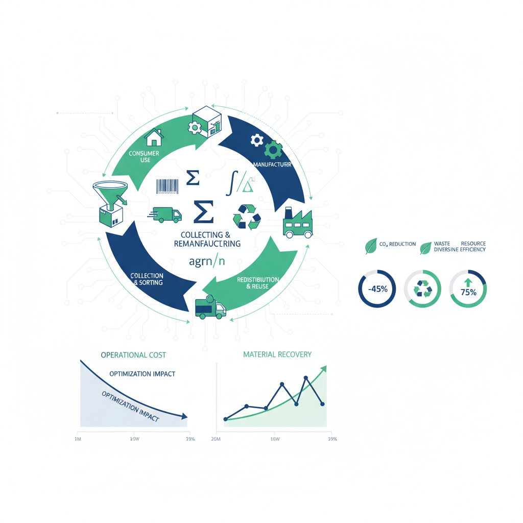
Forward-reverse closed-loop supply chain models integrate product acquisition, recovery center siting, and re-manufacturing scheduling into a unified network design. Research proves that mathematically co-optimizing forward and reverse logistics channels yields overall system cost reductions between 12% and 25% relative to siloed operations 8 .
4. The Future of Operational Research: AI-OR Integration & Quantum Computing
“The best way to predict the future is to create it.”— Peter Drucker, management consultant
The convergence of Artificial Intelligence and Operations Research (AI-OR) is revolutionizing distribution logic:
-
Deep Reinforcement Learning (DRL): Employed to solve Dynamic Pick-Up and Delivery Problems (DPDP) in dense urban grids where real-time traffic invalidates static offline schedules within minutes.
-
Quantum Combinatorial Solvers: Algorithms running on Quantum Annealers (e.g., Quadratic Unconstrained Binary Optimization or QUBO formulations) evaluate global routing possibilities orders of magnitude faster than classical branch-and-bound solvers.
Next Steps: Actionable Roadmap for Implementation
To systematically deploy Operations Research methodologies within corporate logistics infrastructure, execute the following phased roadmap:
-
Phase 1: Network Data Audit & Baseline Formulation
-
Extract granular transaction data (origin-destination matrix, weight, cube, tariffs, historical lead times).
-
Formulate current baseline logistics costs utilizing deterministic linear accounting.
-
-
Phase 2: Mathematical Model Formulation & Solver Setup
-
Build exact Mixed-Integer Linear Programming (MILP) formulations representing real-world facility constraints, throughput capacities, and SLA requirements.
-
Integrate commercial optimization solvers (e.g., Gurobi, CPLEX) or open-source frameworks (e.g., Python SciPy/PuLP).
-
-
Phase 3: Simulation & Sensitivity Analysis
-
Run Monte Carlo simulations against optimized decisions to evaluate resiliency under stochastic demand shifts and supply bottlenecks.
-
Execute dual-variable (shadow price) sensitivity analysis to locate capacity constraints where marginal investment yields maximum operational savings.
-
-
Phase 4: Telematics & Continuous Re-Optimization
-
Establish real-time data feeds connecting fleet telematics directly to routing solvers.
-
Continuously monitor Working Capital release, Working Capital Ratio, and Cash Conversion Cycle metrics to validate ROI against predicted quantitative targets.
-
“Without mathematics, there’s nothing you can do. Everything around you is mathematics. Everything around you is numbers.”— Shakuntala Devi, mathematician and writer